Determining the Eigenfrequencies and Normal Modes of Coupled Pendula

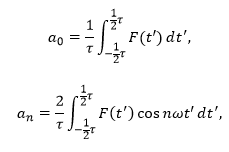
While the motion of a system of coupled oscillators can be very complex, the system’s eigenfrequencies ω and normal mode motion can be determined by applying a fairly simple procedure.  A system’s eigenfrequencies and normal mode motion refers to the natural resonant frequencies of the system and the pattern of motion in which the system undergoes when all parts move with the same frequency, respectively.  To determine the eigenfrequencies and normal mode motion of a system of coupled oscillators:

1.  Formulate the lagrangian equations for the system’s kinetic energy T and potential energy U.
2. Construct A_ij and m_ij tensors in n x n arrays to describe how the system’s various components are coupled.
3.   Form and solve the characteristic equation for ω.  The characteristic equation is given by
   
4. Determine the eigenvectors of the matrix A_ij – ω²m_ij describing the normal mode motion of the system.

Example 1: Two Pendula

Given a system consisting of two pendula of equal length L and mass m connected by a spring of force constant k, we can determine the eigenfrequencies ω and describe the normal mode motion of the system.  Figure 1 illustrates the system.

Figure 1:  This figure shows the system of coupled pendula.  

Image Credit: Classical Dynamics of Particles and Systems by Thornton and Marion

As our pendula only move about the Θ direction and kinetic energy of an object is described by the general equation

where m is mass and v is velocity, the total kinetic energy of our system is

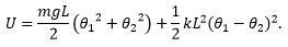
Similarly, as the potential energy of a pendulum and a spring are described by the general equations

and

where g is gravity and x is the distance from equilibrium the spring is either stretched or compressed, the total potential energy of our system is

If we assume our pendula will only undergo small oscillations, we can simplify our potential energy equation using the approximations

and

 Thus, our potential energy is

Next, we construct our A_ij and m_ij tensors.  The components for each of these tensors is determined by the relations

 and

where q_i and q_j represent the respective generalized coordinates.  In this case, the generalized coordinates are simply Θ₁ and Θ₂.  Thus, our tensors are

and 

Next, we form and solve the characteristic equation for ω. Our characteristic equation is given by

meaning we must set the determinant of matrix A-ω²m equal to 0 and solve for ω.  We find the eigenfrequencies of the system are

and

Finally, after solving for the eigenvectors of the system, we determine the normal modes of the system to be

and

This means that our pendula can obtain constant oscillatory motion two ways: by swinging together at equal velocities or by swinging exactly opposite eachother, see Figure 2.

Figure 2:  This figure illustrates the normal modes of the coupled pendula.  

Image Credit: Classical Dynamics of Particles and Systems by Thornton and Marion

Example 2: Three Pendula

Given a similar system to that of example 1 but containing an additional pendulum, we can use the same process to determine the new system’s eigenfrequencies and normal modes.  Below are the respective functions and tensors.

In this case, the pendula can swing together, the outer two can swing in opposite directions while the middle remains stationary, or the outer two can swing together while the middle swings in the opposite direction with an increased amplitude.

Modeling A Bungee Jumper's Motion

Modeling a bungee jump is fairly simple given a basic background in kinematic motion and simple harmonic oscillation.  To begin, we must define a differential equation describing the net force acting upon our jumper throughout the span of their flight.  Assuming the jumper’s motion is entirely in the vertical  direction, we will consider two unique types of motion: free fall and simple harmonic oscillation.  While the jumper’s position resides above the hanging length L of the bungee cord, their motion is described as free fall.  As the jumper falls below the hanging length of the cord, their motion can be thought of as the bottom half of a mass on a spring’s oscillation, see Figure 1.

Figure 1:  This is a simple schematic illustrating the sections described by each type of motion.

In order to construct our differential force function, we must consider the net force upon the jumper during each portion of their flight.  While in free fall, the only forces acting on the jumper are gravity and air resistance, see Figure 2.  When the jumper’s position is lower than L, the jumper is acted upon by gravity, air resistance, and a spring force due to the overstretched bungee cord, see Figure 2.  Here, it is important to note that the retarding air drag force is constantly directed antiparallel to the jumper’s velocity.

Figure 2: These are the two free body diagrams illustrating the forces in each section of motion.  If the direction of the mass's velocity changes, the direction of the drag force will also switch.

We now construct our piecewise differential function

where m is the jumper’s mass, g is gravity, b is the damping coefficient due to air resistance, v is the jumper’s velocity,  and k is the sprint constant of the bungee cord.

In order to simulate a jumper’s motion, we must assign values to our model’s various parameters, see Table 1 for full listing.  As b and k are more difficult to assign, we solve for them instead.  When solving for b, we know that a person in free fall will eventually reach a terminal velocity v_t when the force of air resistance is equivalent to the force of gravity.  Thus, as

we know

An average person’s terminal velocity in free fall is approximately 53 m/s.[1]

Assuming that a bungee cord stretches about 4 times its resting length during a jump and that a jumper experiences approximately 3 G’s at the bottom of the jump [2], we formulate the relationship

Thus,

and 

Table 1: These are the parameters used for the real world simulation.

Finally, the differential F(z(t)) equation can be solved numerically and graphically displayed using Mathematica.  In the case of a real-world bungee jump, the jumper’s motion is qualitatively represented in Figure 3.

Figure 3:  This is a visual of the jumper's motion under real world parameters.  The jumper begins their flight at z=0.

Furthermore, we can test extreme cases to show that the model is qualitatively accurate.  Figure 4 illustrates the case of an extremely high spring constant k value.  Here it is evident that, while the simple harmonic oscillation section of the jumper’s motion is greatly altered, this does not affect the free fall portion of their motion other than propel them to greater heights as the spring force is increased.

Figure 4:  This is a visual of a jumper's motion when the cords spring constant is extremely high.  It is clear that the change in spring constant only alters the initial conditions as the jumper re-enters the free fall portion of motion.

This model could now be expanded to include more dimensions or could be used to prepare for jumps in new locations or under various conditions.

 Sources:

1. http://hypertextbook.com/facts/JianHuang.shtml
2.http://www.bungeezone.com/equip/cord.shtml

Fourier Series

Nearly any periodic function can be represented as a linear combination of simple, sinusoidal waves.  By applying a process known as a Fourier transform, one can represent a complicated periodic function as an approximation displaying each individual component in superposition.

The Fourier transformation process consists of rewriting the original F(t) function in the form of

where n is an integer from 1 to infinity, ω represents angular frequency, t is time, and a₀, a_n, and b_n are coefficients.  To determine the a₀, a_n, and b_n coefficients, it is necessary to evaluate three integrals:

and

After determining each coefficient, the process is completed by plugging each in to its respective place within the Fourier series form of F(t).

Example:

(Problem 3-28 from Classical Dynamics of Particles and Systems 5^th Edition by Thornton and Marion)

Obtain the Fourier expansion for the function

in the interval –π/ω < t < π/ω where ω = 1 rad/s.

Solution:

After plotting the function, we determine that the function is odd as F(-t) = -F(t), or the values on the left and right side of the y-axis are of equal absolute value but opposite in sign.  This means that a₀ must equal 0 as the integral of an odd function of period 2π over the interval –π/ω < t < π/ω is always 0.

So,

Similarly, when determining a_n, we have an odd function F(t) times an even function cos(nωt).  This results in an overall odd function F(t)cos(nωt).  Thus, for the same reasons as a₀,

When determining b_n, we have an odd function F(t) times an odd function sin(nωt) resulting in an overall even function F(t)sin(nωt).  In this case, we must take the integral.

                        

Thus,

or

By plotting the original function and the Fourier expansion including various numbers of terms, it is clear that as the number of terms included in the expansion increases, the Fourier series plot approaches that of the original function.  Below are plots of the original function, the Fourier series including two terms, the Fourier series including three terms, and the Fourier series including four terms, respectively.