Hamiltonians

                While the formulation of a Lagrangian and Lagrange equations of motion can greatly simplify an otherwise complicated system, it is not the only way.  Similarly to the application of Lagrangians described in Hamilton’s Principle and Lagrangians and Lagrangians Pt. 2, the formulation of a system’s Hamiltonian provides easy access to the time depended equations of motion for each generalized coordinate necessary to describe the system.  To begin, we determine the Lagrangian

as before, where q represents the chosen general coordinates and T and U represent the kinetic and potential energies of the system, respectively.  Next, we construct our Hamiltonian equation given by

While I will not be further discussing its derivation, this generalized Hamiltonian equation is the result of a Legendre transform of the generalized Lagrangian.  Here, p_k represents the momentum associated with the respective generalized coordinate q_k.  Furthermore, as the Hamiltionian is a function of q_k, p_k, and t instead of q_k, dq_k/dt, and t as is the Lagrangian, it is necessary that each velocity present within the equation be replaced with an equivalent expression in terms of momentum provided by the relation

Finally, the relations

and

known as the Hamilton equations of motion, provide the system’s 2n first order differential equations.  By applying initial conditions and solving this system of differential equations, time depended equations of motion for each generalized coordinate can be determined.  Below is an example of this process’s application to a simple pendulum.

Example:

(Based on Problem 7.24 from Classical Dynamics of Particles and Systems 5^th Edition by Thornton and Marion)

Consider a simple plane pendulum with a fixed suspension point consisting of a mass m attached to a string of length ℓ. After the pendulum is set into motion, the length of the string is shortened at a constant rate

Determine the Hamilton equations of motion for this system.

To begin, it will be useful to define the length of the pendulum ℓ by integrating over time the rate at which it is shortened.  Thus, we find

where L is the original length of the pendulum.  Next, we determine the pendulum’s Lagrangian.  As

we determine that

where g is gravitational acceleration.  Third, we construct our Hamiltonian equation

but as it must be in terms of momentum rather than velocity, we substitute the relation

Now, with our Hamiltonian

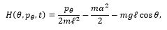
we can determine our Hamiltonian equations of motion

and

Below is an animation of this pendulum’s motion given that L=4.0m, α=0.5m/s, m=1.0kg, g=10 m/s^2, θ(0)=π/4 radians, and θ’(0)=0 radians/s.